Volumetric Time, Minor Quantum Computation State-Preparation and Harmonic Chord Conversion to Linear Operator Matrices: Fundamentals and Methodologies

      The primary aim of this research is to explore the intersection of quantum computing, music theory, and visualization by creating a comprehensive representation of 3-dimensional volumetric-time data about a given point-particle region and its relationship to musical intervals, wavelength, energy levels, and octave pitch classification sets. It will involve the application of quantum logic gates and the Qiskit package, specifically using OpenQASM2.0 in tandem with Q-Ctrl's Fire Opal interface to run experiments on a real quantum computer, courtesy of IBM (Q), to encode volumetric-time information into relatively manageable n>=11 qubit states, as well as the mapping of eigenvalues to musical intervals using quantum algorithms or simulations. It will also include the creation of a 3D scatter plot and geometric topology to visualize the relationships between the data points, with an emphasis on incorporating volumetric time into the visualization. The research will achieve a complex and multi-faceted representation of the data. The intention, curiosity notwithstanding, will contribute to the fields of quantum computing, music theory, and visualization processes by providing a novel approach to representing and understanding multidimensional data in a 3±1-dimensional context.

In other words, this is as much a study as it is a complex thought experiment. Thus far, I have yet to encounter an exploration of these subjects as a collection, not just disparate, barely connected tissue. I chose no more than 11-qubits, excluding the obligatory scratch qubit only because it seemed sufficient for the amount of data that all of this contains and I felt it would be necessary to have bit space to expand if need be without being too nebulous.

Please see the previous posting for the detailed considerations and descriptions of Volumetric time. It's not the simplest concept and it's still in development so it is not something that will be found elsewhere - some confusion [or maybe a lot] should be expected.

The main visualization tools are 'visualization libraries' such as Matplotlib, Plotly and Numpy. Silly names aside, these libraries and Python 3 overall are instrumental to working on any of this, so it is important to spend some time with these powerful digital repositories. So we start with graphing this concept, just to get started. However keep in mind these formats will radically change over the course of this, therefore there is no particular one framework that's best; different strokes and all that.

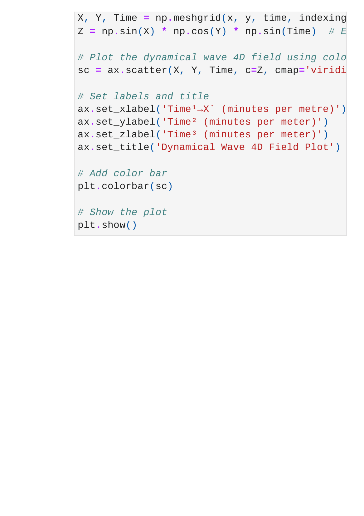
We'll begin by creating a basic representation of a 3 dimensional field, however this will not be the usual Cartesian X,Y, Z coordinate system but instead a field of 3 independent axes of time about a point of space. Essentially a kind of inverted spacetime, 'Timespace'. Neat. For this the units will be irrelevant to set the scene but normally via inverted differential techniques - this can now be regarded as something like "hours per mile", "hour per kilometre", "minutes per metre", et al. Yes, it is weird. Something that helps wash that down with a bag of chips is relegating each axes to be either the imaginary field of the Cartesian space or past, present, future or just simply 'Time 1, Time 2, and Time 3.'

To encode 3-dimensional volumetric-time over a singular position within the qubit states using quantum logic gates, we can use the concept of quantum state encoding and manipulation. We'll need to use a quantum circuit to perform the encoding. We can use the Qiskit package, which is an open-source quantum computing framework for writing quantum circuits. Here's a high-level overview of the steps involved:

Create a quantum circuit with sufficient qubits.

Encode the 3-dimensional volumetric-time information over a singular position within the n>=11-qubit states using quantum logic gates.

Apply the necessary quantum gates to manipulate the qubits to represent the desired information.

The actual setup is more involved than this but that aspect is built in enough that once you grasp the language of quantum dynamics and computational considerations of the field, then the starting point will be further along than the very beginning every time. See previous entries for that part, mainly the Tonal-Harmonic theory book or visit IBM's website.

The quantum framework has been set up and now we can freely correlate these states and gates with the graphing process, creating a graph that maps eigenvalues to music intervals with various octave-pitch classifications and energy levels based on Planck's constant and the wavelength of the absolute note values; a fascinating intersection of quantum mechanics and music theory. The following time graph has been prepared in a state of superposition, similar to the former but its been polarized and carries different aspects of the data. Ideally, it is wise to super impose each one of the other to form the more realistic but inherently noisier state. This will need to be tuned using the quantum gates in order to preserve the information sufficiently. To accomplish this, you can follow these general steps:

Calculate Eigenvalues, using quantum algorithms or simulations to calculate the eigenvalues of a quantum system, such as a molecular Hamiltonian representing a musical note.

Map Eigenvalues to Music Intervals, calculate eigenvalues to musical intervals using a suitable mapping function. For example, you can map the eigenvalues to specific musical intervals based on their relative energy levels or orbital electron shells.

Incorporate Octave Classifications, consider the octave classifications and map the musical intervals to their respective octave classifications based on their frequencies within the general pitch class sets.

Calculate Energy Levels using Planck's constant and the wavelength of the absolute note values to calculate the energy levels associated with each musical interval.

Create a Graph so as to visualize the mapped eigenvalues, musical intervals, octave classifications, and energy levels in a graph or chart.

Here's a simplified example of how you might approach this:

Map the eigenvalues to musical intervals, incorporate octave classifications, calculate energy levels based on Planck's constant and the wavelength of the note values, and create a graph to visualize the mapped data. In this example, we create a 3D scatter plot to visualize the relationship between eigenvalues, musical intervals, octave classifications, and energy levels. The x-axis represents musical intervals, the y-axis represents octave classifications, and the z-axis represents the calculated wavelengths. The color of the points represents the energy levels associated with each data point.

This visualization provides a conceptual representation of the relationship between the eigenvalues, musical intervals, octave classifications, and energy levels in a 3-dimensional context.

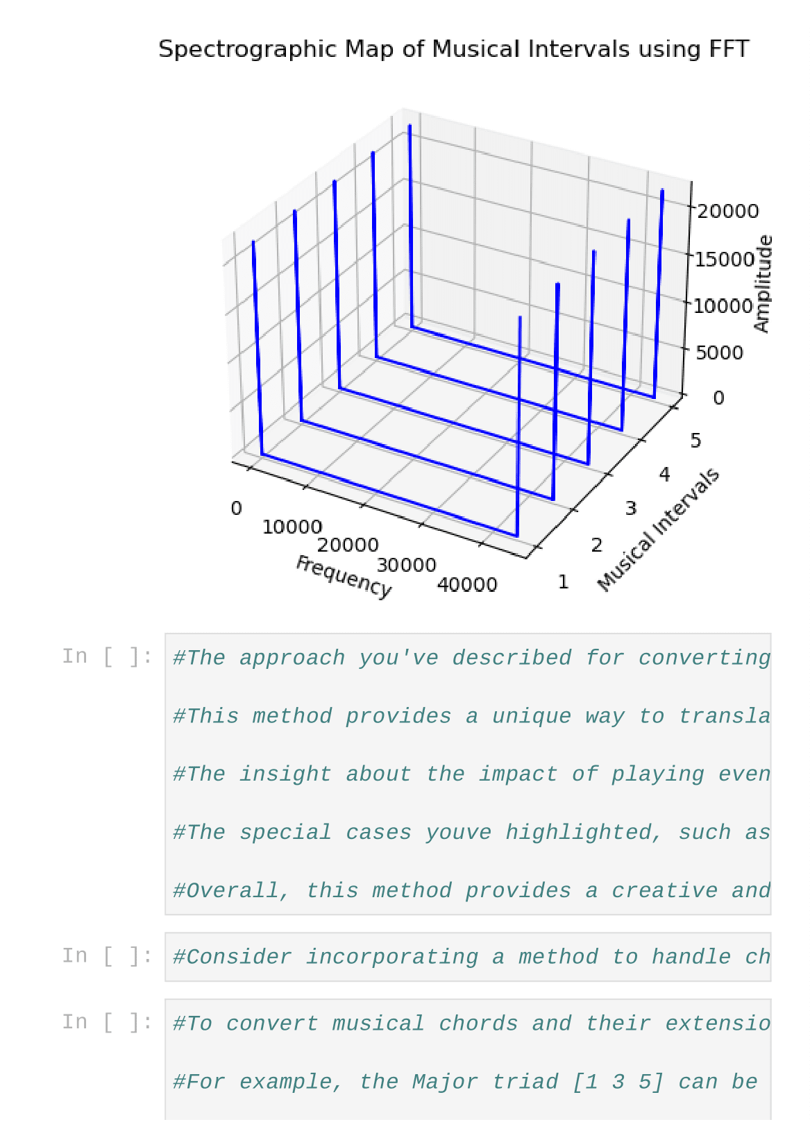
Creating a spectrographic 3D map of musical intervals correlated to wavelength, Planck's energy levels, octave pitch classification, and corresponding 3 dimensions of volumetric time, along with a complementary wireframe with the nodes as musical intervals, is a complex and multi-faceted task that involves integrating concepts from quantum mechanics, music theory, and visualization.

Spectrographic 3D Map:

Use a 3D scatter plot to visualize the relationship between musical intervals, wavelength, Planck's energy levels, and octave pitch classification. Each data point in the scatter plot represents a musical interval, with its position determined by the wavelength, energy level, and octave classification.

The color of the data points can represent the energy levels associated with each interval.

Geometric Wireframe:

Create a wireframe with nodes representing the musical intervals. For modal invariant notes of a scale, fill in the corresponding nodes to highlight their significance within the scale.

Wireframe geodesics can be constructed using a library such as Matplotlib or Plotly to create a 3D representation of the musical intervals.

Incorporating Volumetric Time:

If representing 3 dimensions of volumetric time, consider incorporating time as an additional dimension in the 3D scatter plot or wireframe visualization. This could involve using animation or color gradients to represent the evolution of the musical intervals over time.

There's that 'Time-Matter Particle-Wave Quadruplicity' again..neat.

.The approach you've described for converting a chord into a time signature is a fascinating and creative concept that combines music theory and mathematical principles. By summing the intervals of a chord and adjusting for sharps and flats, you derive an integer that can be rounded to the nearest subdivision to create a time signature.

#This method provides a unique way to translate musical elements into rhythmic structures, allowing for the creation of complex and compound time signatures based on chord qualities. The idea of combining different chord qualities to derive complex time signatures is particularly intriguing and offers a novel approach to rhythm composition.

#The insight about the impact of playing even-ordered time signatures last in a sequence to create a smooth rhythm, and odd-ordered time signatures last for a more asymmetrical rhythm, adds an additional layer of musical interpretation and performance considerations.

The special cases highlighted, such as the summed integer of 6 and 1, and the unique treatment of 1/1 as a special placeholder function in a time signature cadence, demonstrate the depth and flexibility of this approach.

Overall, this method provides a creative and innovative way to bridge the gap between music theory and rhythmic structure, offering a new perspective on the relationship between chords and time signatures. It opens up possibilities for experimentation and artistic expression in musical composition and performance.

Consider incorporating a method to handle chord inversions, as they can affect the interval sums and subsequently the derived time signatures. To convert musical chords and their extensions into algebraic linear operator matrices, we can represent each note in the chord as a vector in a complex vector space. The flat tones can be represented as the integer minus an imaginary variable, and sharp tones can be represented as the integer plus an imaginary variable; that is i or j. Where either i=j, or i=negative condition of the variable and j=positive condition of the same variable. It's just a notational different for certain tasks or complexities when mixing and matching different chords, likely from different pitch class sets or some comparable analysis/practice.

For example, the Major triad [1 3 5] can be represented as the vectors [1, 3, 5] and the Half-Diminished 7th chord [1 b3 b5 b7] can be represented as the vectors [1, 3-i, 5-i, 7-i]...

To perform operations such as multiplying two chords, we can represent each chord as a matrix and then perform matrix multiplication to obtain the result.

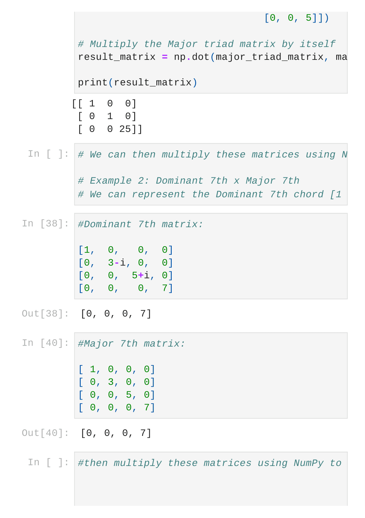
Lets take the example of multiplying the Major triad [1 3 5] by itself:

The Major triad [1 3 5] can be represented as the following matrix:

| 1 0 0 |

| 0 3 0 |

| 0 0 5 |

.For the Half Diminished 7th x Major 7 example, we can represent the chords as matrices and then perform matrix multiplication to obtain the result.

10) #In Python, we can use the NumPy package to perform matrix operations. Here's an example of how you might represent and multiply the Major triad [1 3 5] by itself using NumPy:

11) #For the Half Diminished 7th x Major 7 example, you would similarly represent the chords as matrices and then perform matrix multiplication

12) #Let's consider a few more examples of converting musical chords and their extensions into algebraic linear operator matrices and performing operations on them.

Example 1: Major Triad x Minor Triad

We can represent the Major triad [1 3 5] and the Minor triad [1 b3 5] as matrices and then perform matrix multiplication to obtain the result.

| 1 0 0 | |1 0 0 |

| 0 3 0 | x |0 3-i 0 |

| 0 0 5 | |0 0 5 |

Maj Triad x Min Triad; i=//=j here.

(We can then multiply these matrices using NumPy to obtain the result.)

Example 2:

Dominant 7th x Major 7th

We can represent the Dominant 7th chord [1 3 5b 7] and the Major 7th chord [1 3 5 7] as matrices.Then multiply these matrices using NumPy to obtain the result.

In another example, Diminished 7th x Half-Diminished 7th.

We can represent the Diminished 7th chord [1 3b 5b 7bb] and the Half Diminished 7th chord [1 3b 5b 7b] as matrices and then perform matrix multiplication to obtain the result.

which can be rewritten as simply,

| 1 0 0 0 |

| 0 3j 0 0 |

| 0 0 5j 0 |

| 0 0 0 7jj|

;i=j here.

Extend the method to represent chord inversions and voicings as variations of the base chord matrices. This would allow for a more comprehensive representation of different chord voicings and their interactions.

Explore the use of probabilistic models to capture the statistical relationships between chords and their occurrences in musical compositions. This could involve using techniques from machine learning and statistical analysis to model chord progressions and transitions.

Expand the method to incorporate timbral and textural elements of chords, such as instrument-specific characteristics and sound textures. This could involve representing timbral features as additional dimensions in the matrix representation.

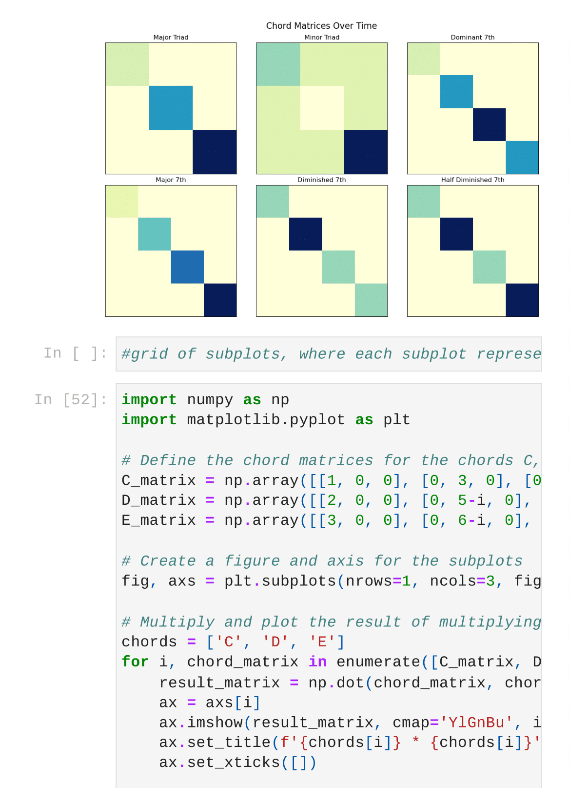
This is a grid of subplots, just to show you how ridiculous this rabbit hole goes, where each subplot represents a chord matrix, and the position of the subplots represents the time or index. This would provide a visual representation of the chord matrices over time.

Here is a chart involving multiplying the chord matrices for the chords C, D, and E major.

Another chart involving multiplying the chord matrices for the chords Cm9, D b13, and Em6 add 9, no 5 and no 7.

The final set multiplies each chord matrix by its adjacent matrix and creates a chart for the results. You can modify the chord matrices and their operations as needed for your specific use case. So cool, right?!

It's the distribution of chord tones across pitch class sets for each chord and its adjacent multiplication. It provides an eerily satisfactory, yet, equally comprehensive view of how the chord tones are can be correlated and permitted to be perceived about the suitable regions of transition between adjacent chords across different octaves ranges.

In conclusion, the exploration of chord matrices and their dynamical properties about a point under time provides valuable insights into the harmonic relationships between chords and how the function that is time maybe translated as the background or the foreground of the dimensionality of massivity or masslessness. By visualizing the multiplication of chord matrices and considering the distribution of chord tones across different octaves, we can gain a deeper understanding of how chords interact and transition within musical compositions as well as the independent, timbrely-affected intervals. This approach not only offers a unique perspective on chord analysis but also demonstrates the potential for leveraging data-driven techniques to uncover new insights in music theory and composition, whether that be the composition of music or the composition of the underlying physics that permits all of these amazing parameters to happen. As we continue to explore the intersection of music and data analysis, there are boundless opportunities to further enrich our understanding of musical structures, quantum phenomena and patterns.

{Quantum Computational Analyst/IBM-Q-Ctrl

Audio and Acoustic Engineer/Conservatory of Recording Arts and Sciences

Music Theorist and Artist/This City Called Earth project

Volunteer 3d Printer Technician/San Diego Public Library - IDEA labs}